Solutions
Asset Liability Management (ALM)
Main Tasks
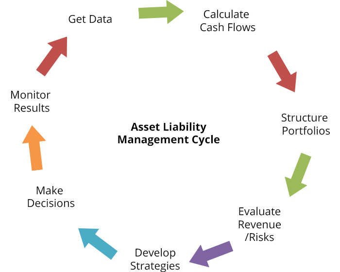
The main objective of Asset Liability Management (ALM) is to effectively hold asset and liability portfolios along the time axis and optimize the RORAC (Return/Risk), using various evaluation and strategy approaches. Due to the complexity of sophisticated mathematical models, effective finance management implies the application of software tools and systems. Our solution accomplishes the following:
- Modeling and pricing of various instrument types.
- Hierarchical structuring of portfolios in assets, liabilities, off-balance positions and their sub-portfolios, using lists, filters and structures.
- Generation and evaluation of cash flows (fixed, float, pay-offs).
- Definition of regular and irregular future periods to be used for ALM analysis.
- Calculation of prices and measures (e.g. Net Present Value) on position level and aggregation on portfolio level.
- Modified duration, convexity, dispersion, internal rate of return, etc..
- Calculation of opportunity rates based on interest rate expressions that can define rates, such as floater, spread, step-up/down, maturity mixed, curve mixed, currency mixed, historical, average, depressed, etc.
- Definition and usage of future scenarios for market factors (FX, interest rates, stock indexes, yield curves, etc.) and for capital development (liquidity scenarios), including prolongation, increase/decrease of business, losses of defaulted debtors, budget plans, future cash flow obligations, etc. The usage of market and liquidity scenarios enables future assessments and stress tests of assets and liabilities. The involvement of simulated positions in the portfolio is a flexible way of planning and investigating future cash flows.
- Performance of advanced ALM analysis, related to future interest and capital developments and transformations, including:
- Cash flow analysis and GAP-analysis for future periods, according to cash flow types, such as capital decrease/increase, interest rate payments, expectated pay-offs of stochastically modeled instruments.
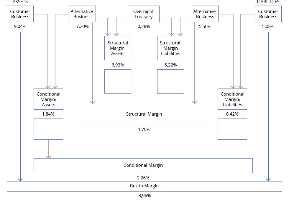
- Interest income analysis that calculates interest rates, margins and contributions for the asset and liability side, based on rates of alternative or market relevant business. Gross, conditional and structural margin and contribution are obtained between the asset and the liability side.
- Fund Transfer Pricing (FTP), that calculates the market value and contributions of assets and liabilities, based on opportunities for alternative businesses with different contract maturities. This functionality is known as maturity transformation, i.e. long-term loans with high interest rates are refinanced by short-term rollover deposits with lower interest rates.
- Refinancing and reinvestment, including the definition of planned positions in order to refinance or reinvest future cash flows.
- Replication of portfolios, used to model future financial instruments without knowing the cash flows or pay-offs, such as rollovers and non-term liabilities.
Calculation Structure and Data Flow
The calculation structure indicates the separate management of the asset and liability side, so that interest rates, opportunity rates, conditional margins and corresponding contributions are calculated in two dimensions:
- Along future periods, as defined by the analytical scheme; e.g., daily during the first week, weekly during the first month, monthly during the first year, etc. The results can be aggregated within the analytical scheme, for example, for the first three months.
- Along the sub-portfolio hierarchy, by aggregating on every sub-portfolio level.
Calculation of FTP results, i.e. structural margins and contributions for assets, liabilities as well as the differences between them, is performed in the next step, where the split between assets and liabilities is based on unit interest rates, e.g. on three-month Libor, or some Overnight Treasury rate.
Asset and liability modules use input data from external and internal databases, user inputs, downloaded market data and internal calculation results for financial instruments. Input data and results are stored into the database for subsequent reporting. The general scheme of the data flow in ALM follows the main steps of data preparation and processing:
- Importing position and instrument data via standard importer.
- Accessing market data (e.g. curves, FX rates, indices) from the client’s core database or via providers.
- Defining lists, filters and structures needed for portfolio structuring.
- Configuring settings, financial calendar, nomenclatures, scenarios, time schedules and opportunity rate definitions.
- Running position and portfolio calculations, as well as ALM analyses, including the aggregation of results and scenarios. Storing the results into reporting database tables.
- Reporting the results in different formats:
- Export to Excel;
- Standard reports: Crystal report, Jasper report, Oracle reports;
- Special reports: OLAP reports using QlikView;
- Regulatory reports: COREP, XML/XBRL output, WEB Browser presentation.
Functionality
Cash Flow Types
| Capitals | |||
| Interest rates | Fixed | Stochastic | |
| Fixed | Credits with fixed interest rate | Credit with an amortization option | |
| Floating | Credits with floating interest rate | Floating certificate of deposit | |
| Stochastic | Deposits with future interest rate agreements |
|
|
ALM deals with interest rate and capital cash flows and pay-offs in future periods. Depending on the interest rate type, fixed and float cash flows can be considered. A stochastic component is included in case of options, representing expected cash flows and distributions.
Market Environment
All modules, including ALM, provide means to manage the market environment, e.g.:
- Instrument prices and dividends;
- Yield curves, credit spread curves and indexes;
- FX rates;
- Stock indexes;
- IB rates;
- Implied volatility;
- Bond future baskets;
- Life table for insurance instruments;
- Application of multiple markets and providers.
Market and Liquidity Scenarios
ALM analysis can be performed under scenario and stress test conditions. Market scenarios define supposed changes in market variables, such as interest rates, exchange rates, prices and indexes of market environment.
Liquidity scenarios include the definition of future developments, reinvestments or refinancing strategies that represent expectations of future changes in cash flows, prolongation of instruments and payments, increases/decreases of business volume, expected and unexpected losses at debtor bankrupts, etc. Liquidity scenarios can also depict budgets and financing plans. In the analysis, one can see the gap between the portfolio’s future without scenarios and the expectations of its future behavior. This is represented via planned synthetic positions at assumed future market conditions. Original portfolios are calculated together with synthetic positions. The results are then used to make decisions at the present point about their future behavior.
Every ALM scenario can combine market and liquidity scenarios.
ALM Analyses
ALM analysis provides means to present future cash flow dispositions and detects any gaps or investment efficiencies in the presence of different market scenarios. Different future behavioral changes (growth, defaults of large customers, deposits increase, etc.) may be activated in cash flow scenarios in order to optimize the asset and liability management.
| Analysis | Functionality |
|---|---|
|
|
|
|
|
|
| Supporting Modules: | Definition of opportunity rates, interest rate expressions, market and liquidity scenarios, analysis by periods and time schemes, static and dynamic portfolio structures and sub-portfolios |
Interfaces and Connectors
The ALM Module inherits the features of Risk Framework Interfaces and Connectors, including:
- Import of data from external sources using flat files.
- COREP reporting for regulatory results, Crystal reporting tool.
- Export / import of interfaces to MS Windows directly and via Clip Board.

